Blogs
Upcoming OpenPIV c++ Optimizations
Introduction
When processing large quantities of PIV images on consumer hardware, it may be often advantageous to provide optimized code paths to accelerate processing. For instance, if it takes five seconds to process a 12 MP PIV image pair and there are 10 batches of 100 image pairs, it would take approximately one hour and 23 minutes to process. If an optimized code path reduces that processing time to something along the lines of two seconds, the overall processing time is reduced to around 33 minutes. This is even more important when using parallelism to take advantage of hardware resources. As such, certain functionalities of OpenPIV-Python has been ported to a c++ library and binded using pybind11 to remain easy to use in a Python environment.
Implentations
As an initial push towards fast and efficient PIV software, the core algorithms of OpenPIV-Python has been ported into c++ and wrapped with pybind11 to provide native Python behaviors. This includes:
Interpolation:
- lagrange interpolation (k=1-5; substitute for spline interpolation)
- lanczos (k=3,5; currently c++ only)
- sinc (k=3,5; currently c++ only)
Deformation
- forward
- symmetric
Cross Correlation
- circular
- linear
- normalized square error (currently c++ only)
Peak Search
- 2 peaks
- 3 peaks (currently c++ only)
Subpixel Estimation
- Gausian (3 point)
- parabolic (3 point)
- centroid (3 point)
- Gaussian (3x3; currently c++ only)
Correlation Statistics
- signal to noise
- peak to peak
Validation
- global threshold (u and v)
- standard deviation theshold (u and v)
- median theshold (u and v)
- normalized median theshold (mag)
- difference threshold (u an v; currently c++ only)
Optimizations
Implementing PIV algorithms in c++ (and later Numba) provides a slew of techniques that can be used to increase performance. For one, the PIV cross correlation algorithm itself is embarrassingly parallel which means each correlation window is independent of all other windows. A basic optimization technique is to parallelize the cross correlation algorithm by splitting correlation windows into stacks and processing each stack in a thread. For instance, if a computer supports 16 threads through hyperthreading, all correlation windows can be broken down into 16 stacks of windows and processed independently. While this is great for ensemble averaged correlations, multithreading is not that efficient. As such, a better yet parallelization technique is multiprocessing where each PIV image is processed on its own process. For a lack of better words, the same 16 threads can process 16 PIV images in parallel. This presents a very efficient means for performing PIV as long as each PIV image pair is independent (e.g., no temporal or ensemble information).
Another area of optimization are interpolation algorithms. Interpolation kernels, especially those that use trigonometry function such as sin, can be quite slow. A basic way to increase interpolation performance is multithreading since each kernel is independent of all other kernels (yet again, embarrassingly parallel). However, multithreading should not be used in conjunction with multiprocessing, so other optimization techniques can also be deployed. A simple, yet elegant way of significantly increasing the performance of interpolation algorithms is through the use of lookup tables. By descritizing interpolation node offsets and using linear interpolation to reconstruct the weights, the different weights of an interpolation kernel can be precomputed. This offloads the high computational complexity of trigonometry functions or other complex interpolation weighting schemes to lookup tables and reduces the amount of operations performed per pixel or vector. As far as the author's knowledge, this is the first time open source PIV software has employed this optimization technique.
Benchmarking
Interpolation
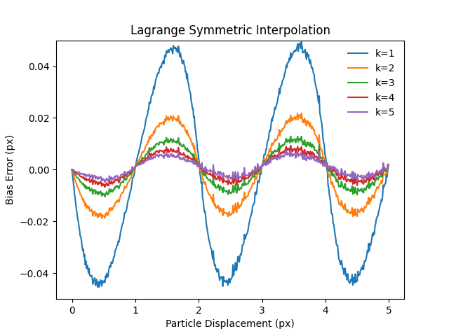
As seen below, the increasing the interpolation order decreases error at the expense of computational complexity. For clarification, all units are in pixels for all images plotting errors.
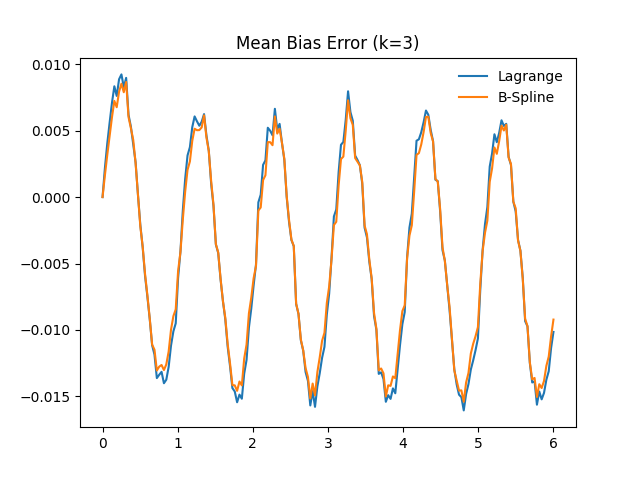
As a sanity check, the interpolation errors are also checked against SciPy's bspline interpolation algorithm (ndimage.map_coordinates) which was used as a baseline throughout development.
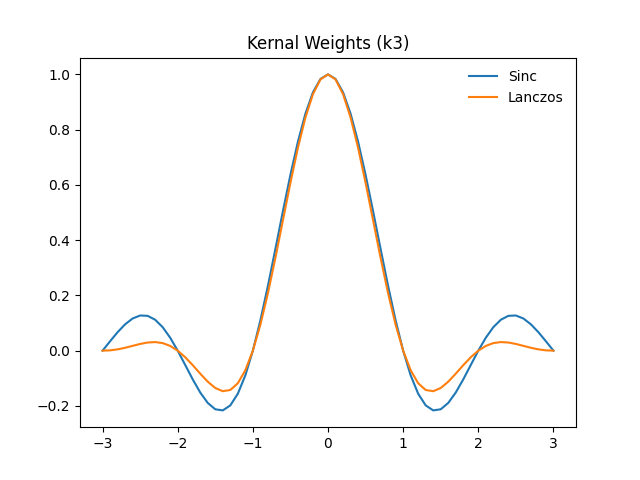
In comparison to OpenPIV-Python, two other interpolation algorithms were implemented: lanczos and sinc. Lanczos is basically a windowed sinc function due to sinc having a near-infinite kernel width due to perpetual oscilations. Both perform better than lagrange or bspline interpolation for particle sizes on the orders of two to four pixels. For a visual representation, the kernel weights are plotted below.
Cross Correlation
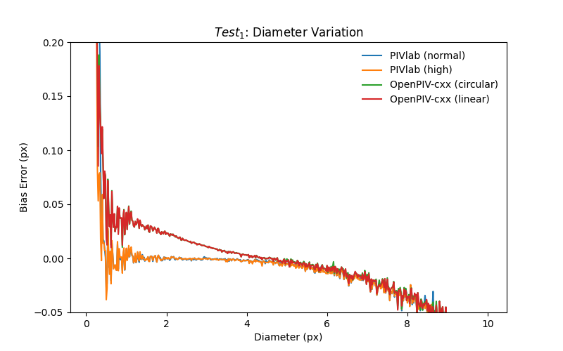
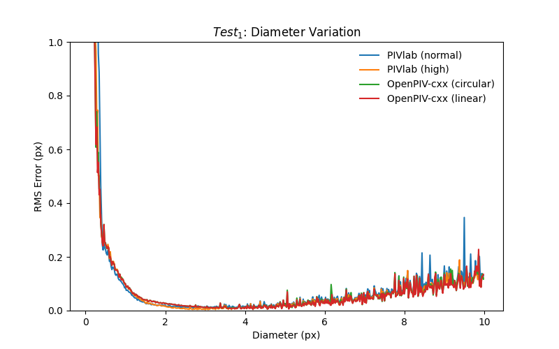
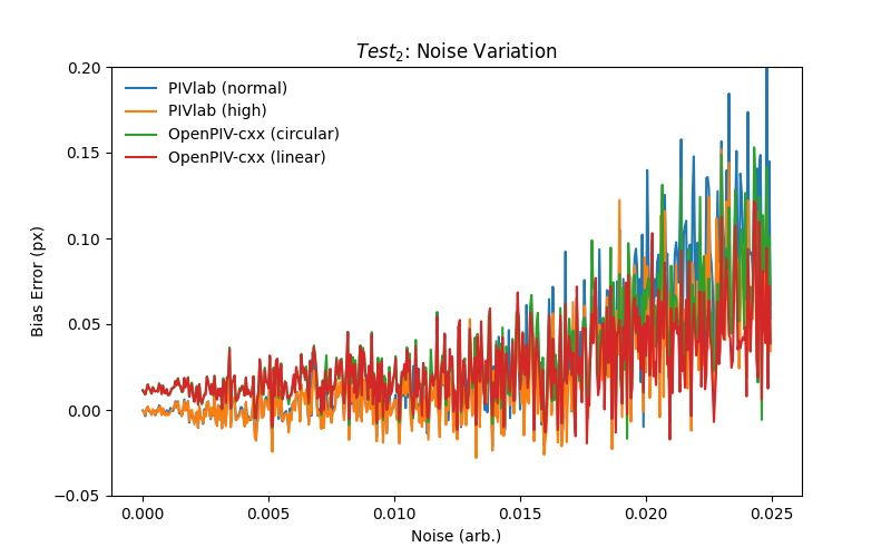
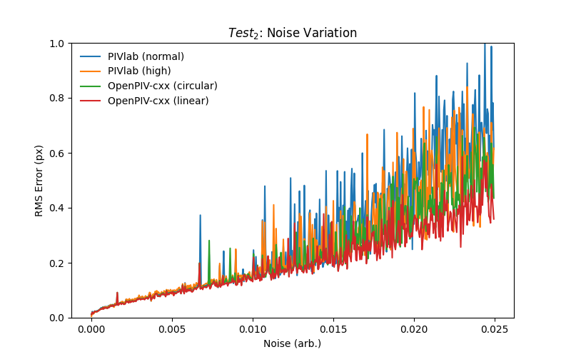
To analyze the performance of the new enhancements to the c++ version of OpenPIV, a basic recreation of the benchmark tests performed by William Thielicke at Optolution had been performed. The results of his benchmark on the performance of PIVlab can be seen here. A series of 9 batches of PIV images, each containing 500 image pairs, were created to test the effects of noise, particle size, and displacements on PIV images. Each batch is characterized in the table below. Batches without a specified particle density are assumed to have a particles per pixel (ppp) ratio of 0.05 and mean particle diamter of 3 pixels.
| Batch # | Test Type | Conditions |
|---|---|---|
| Batch 1 | Particle size test | 0 pixels to 10 pixels; 2.5 pixels displacement |
| Batch 2 | Noise test | 0% noise to 25% noise; 2.5 pixels displacement |
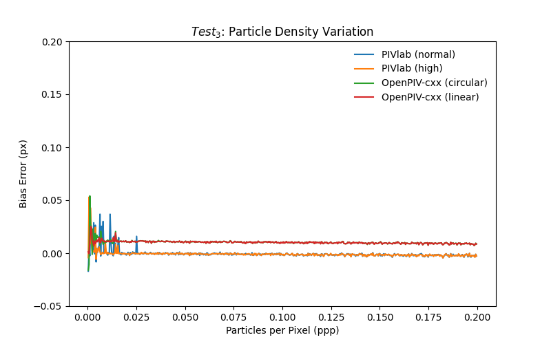
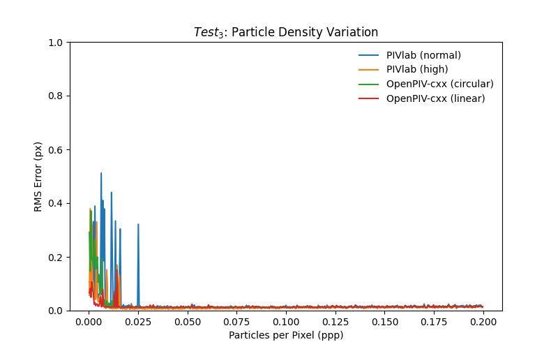
| Batch 3 | Particle density test | 0 ppp to 0.2 ppp; 2.5 pixels displacement |
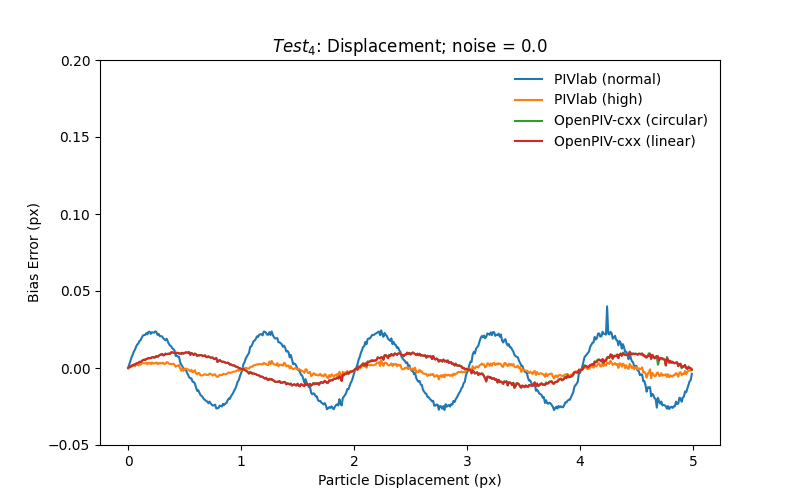
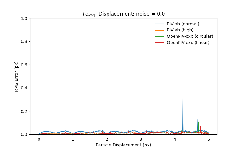
| Batch 4 | Displacement test | 0.000 noise; 0-5 pixels displacement |
| Batch 5 | Displacement test | 0.005 noise; 0-5 pixels displacement |
| Batch 6 | Displacement test | 0.010 noise; 0-5 pixels displacement |
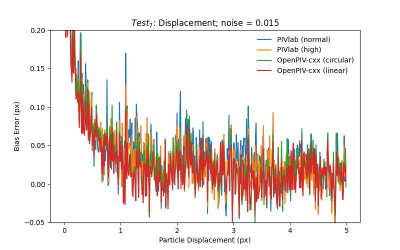
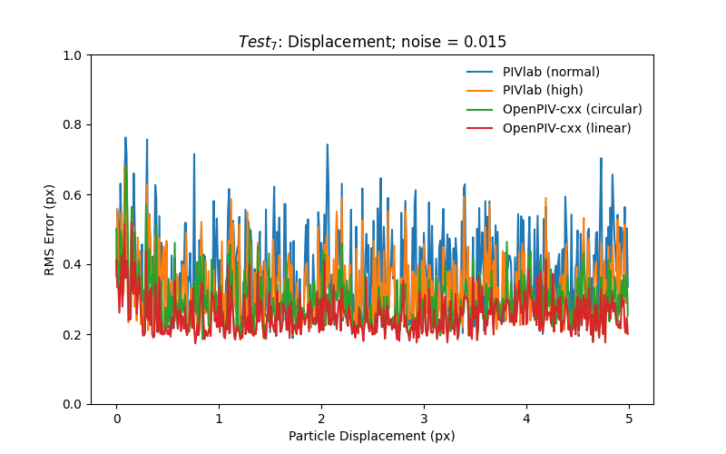
| Batch 7 | Displacement test | 0.015 noise; 0-5 pixels displacement |
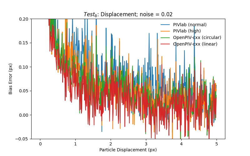
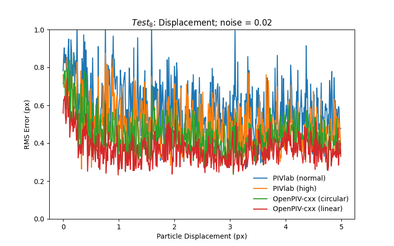
| Batch 8 | Displacement test | 0.020 noise; 0-5 pixels displacement |
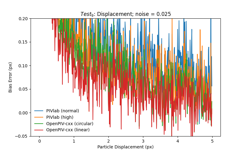
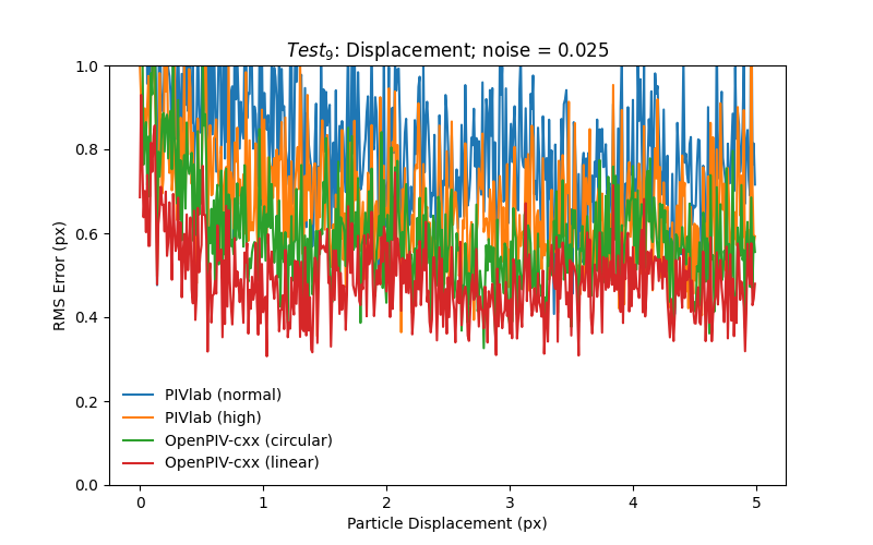
| Batch 9 | Displacement test | 0.025 noise; 0-5 pixels displacement |
During the tests, some amends were made. For one, particle diameters had a standard deviation of zero for test batches one through three to minimize variables. Batches four to nine still have a standard deviation of one pixel (e.g., particle sizes of 3 +/- 1 pixels). Finally, particle loss was removed from the noise tests due to certain concerns observed during the results, which seemed to not be a problem.
PIV Settings
Note: No preprocessing or postprocessing was done on any image pair.
PIVlab (normal):
| Setting | Value |
|---|---|
| IW Sizes | 64 -> 32 -> 24 |
| Overlap Sizes | 32 -> 16 -> 12 |
| Zero Padding | None |
| Interpolation | Linear |
| Deformation Order | 1 (forward) |
PIVlab (normal):
| Setting | Value |
|---|---|
| IW Sizes | 64 -> 32 -> 24 |
| Overlap Sizes | 32 -> 16 -> 12 |
| Zero Padding | 2N - 1 |
| Interpolation | Spline (k=3) |
| Deformation Order | 1 (forward) |
OpenPIV (circular)
| Setting | Value |
|---|---|
| IW Sizes | 64 -> 32 -> 24 |
| Overlap Sizes | 32 -> 16 -> 12 |
| Zero Padding | None |
| Interpolation | Lagrange (k=3) |
| Deformation Order | 2 (symmetric) |
OpenPIV (linear and robust)
| Setting | Value |
|---|---|
| IW Sizes | 64 -> 32 -> 24 |
| Overlap Sizes | 32 -> 16 -> 12 |
| Zero Padding | 2N |
| Interpolation | Lagrange (k=3) |
| Deformation Order | 2 (symmetric) |
PIVview
| Setting | Value |
|---|---|
| IW Sizes | 64 -> 32 -> 24 |
| Overlap Sizes | 32 -> 16 -> 12 |
| Zero Padding | None |
| Interpolation | Spline (k=3) |
| Deformation Order | 2 (symmetric) |
Results
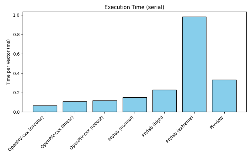
The results from the benchmark can be seen below. An immediate difference can be seen between OpenPIV-cxx's symmetric deformation and PIVlab's forward deformation. This is especially noticable on tests 1-3 where the particle displacement is located at the peak error of the interpolation's frequency response whereas forward deformation has a minimum error at this displacement. When using forward deformation for OpenPIV-cxx, tests 1-3 converge quite neatly showing the effectiveness of the lagrange interpolation as a substitute to basis splines. In general, zero padding the interrogation windows to remove periodic signals from the fast fourier transforms decreased bias and RMS errors. This can also be seen in PIVlab's high setting. As such, the c++ implementation appears to be in agreement with PIVlab (which is sometimes more accurate/precise than commercial software) in regards to this specific benchmark suite. Finally, a the time per vector for PIVlab, OpenPIV-cxx (with FFT SIMD optimizations), and the venerable PIVview software can be seen in the final figure. Through these benchmarks, many optimizations have been made to OpenPIV-cxx to improve its memory efficiency, thus improving it's performance significantly and to the level of Matlab optimizations.
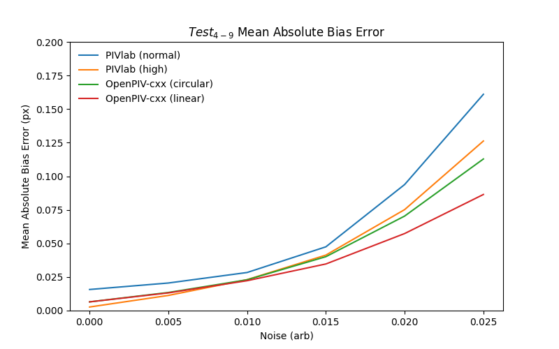
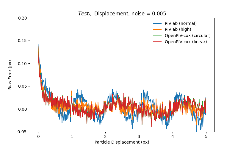
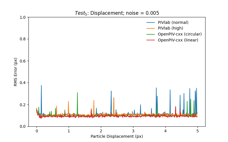
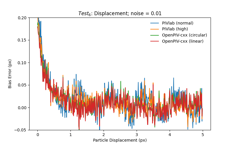
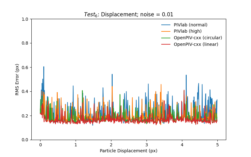
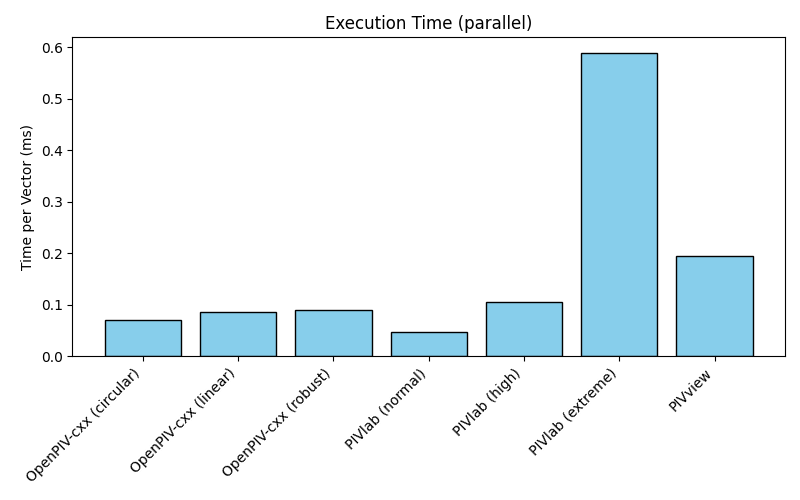
A notable mention should be made for the parallel tests. PIVlab used 8 parallel processes (workers) with each processing their own image pairs. This is the most efficient form of distributed processing for PIV images that are not time-resolved. Contrarily, PIVview and OpenPIV-cxx used multithreading with 8 threads processing the same image pair. This is a lot less efficient compared to distributed processing, as seen in PIVlab's performance.